Traditional Forecasting methods using R

A particular method of examining a set of data points gathered over a period of time is called a "Time series analysis." Instead of just capturing the data points intermittently or arbitrarily, time series analyzers record the data points at regular intervals over a predetermined length of time. But this kind of study involves more than just gathering data over time.

It is like a group of observations of clearly defined data points produced over time via repeated measurements. A time series might include, for instance, calculating the number of retail sales for each month of the year. In this tutorial, you will learn the time series techniques by using the R.

An attempt to anticipate the future value of a single stock, a certain market sector or the market overall is known as a stock prediction. Stock is the best example to demonstrate the time series forecasting technique. Here, we will try implementing Navie, Simple exponential Smoothing, ARIMA and Holt's trend. Let us suppose that the series contains seasonal variation then we can use seasonal navie or TBATS models to predict future outcomes.

Apple stock price is used here to demonstrate the time series forecasting model and the data is taken from "Yahoo Finance". The data is about 22 years of Apple stock value (close price) monthly wise manner which contains 264 rows with 6 variables. But only one variable is used to forecast in the univariate time series forecasting model which is why the closing price has been selected because the closing price is the next day's opening price. 

Then let's see the packages required to perform the traditional forecasting methods in R:

library(readxl)
library(urca)
library(lmtest)
library(fpp2)
library(forecast)
library(TTR)
library(dplyr)
library(tseries)
library(aTSA)

Reading the data from the Excel file (.xlsx) and checking the structure of the data frame.

AAPL = read_excel("/file_path/AAPL.xlsx")
str(AAPL) # To check the structure of the dataframe

For any model, first of all, we have to divide the dataset into training data and testing data. Usually, 80 per cent of the data is used to train the model and 20 per cent of the data is used to test the model. Here, we divided the dataset into train and test as a class.

class = c(rep("TRAIN", 211), rep("TEST",53)) # creating the TRAIN and TEST as class varible

str(class)

AAPL = cbind(AAPL, class)    # Binding the "class" column with the existing AAPL data frame
AAPL

# Splitting the data
train_data = subset(AAPL, class == 'TRAIN')

test_data = subset(AAPL, class  == 'TEST')

Then we have to convert this data into time series by using the "ts" command as shown below.

dat_ts = ts(train_data[,5], start = c(2000,1), end = c(2017,07), frequency = 12)
dat_ts

The output of the model shows the error measure for only the training data but we want the predicted values from the trained model and the test data should be used for the error measure. so we have to define the functions for error measures.

mae = function(actual,pred){

  mae = mean(abs(actual - pred))

  return (mae)
}

RMSE = function(actual,pred){

  RMSE = sqrt(mean((actual - pred)^2))

  return (RMSE)
}

Forecasting models:

Navie Model

nav = naive(dat_ts, h = 53)
summary(nav)

df_nav = as.data.frame(nav)

mae(test_data$Close, df_nav$`Point Forecast`)
RMSE(test_data$Close, df_nav$`Point Forecast`)

OUTPUT

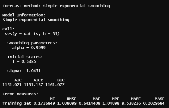
Simple Exponential Smoothing

se_model = ses(dat_ts, h = 53)
summary(se_model)

###

df_s = as.data.frame(se_model)

mae(test_data$Close, df_s$`Point Forecast`)
RMSE(test_data$Close, df_s$`Point Forecast`)

OUTPUT

Holt's Trend Method

holt_model = holt(dat_ts, h = 53)

summary(holt_model)

####
df_h = as.data.frame(holt_model)

mae(test_data$Close, df_h$`Point Forecast`)
RMSE(test_data$Close, df_h$`Point Forecast`)

OUTPUT

ARIMA

The "auto.arima" will select the order automatically for the time series and here we used the Akaike information criterion (AIC) criteria to select the best model for the time series as shown below.

arima_model_AIC = auto.arima(dat_ts,stationary = FALSE, seasonal = FALSE, ic = "aic", stepwise = TRUE, trace = TRUE)

summary(arima_model_AIC)

###
fore_arima = forecast::forecast(arima_model_AIC, h=53)

df_arima = as.data.frame(fore_arima)
df_arima

mae(test_data$Close, df_arima$`Point Forecast`)
RMSE(test_data$Close, df_arima$`Point Forecast`)

OUTPUT

If you wanna get the graph of all the models with the plots, you have to use the below code:

par(mfrow=c(2,2))
plot(nav)
plot(se_model)
plot(holt_model)
plot(fore_arima)

OUTPUT

Conclusion

The performance of the models is measured by the error measures and those are summarized below:

METHODS	MAE	RMSE
Naive Method	43.46769	59.85306
Simple Exponential Smoothing	43.46781	59.85314
Holt’s Trend Method	38.83641	54.82537
ARIMA	39.33623	55.23373

From this table, Holt's Trend method has the lowest Mean Absolute Error (MAE) and Root Mean Squared Error (RMSE) so it is best than other models. Here we just compare the models with the error measures. From this, we can't say that model will definitely predict the exact future value but it will predict the future value with this amount of error. 

To view the overall source code as R markdown!!!! -

NOTE: This post is all about some of the basic models of traditional forecasting methods, the clear explanations of the models are in the book "Forecasting Principles and Practice".